Multiprocessing

---

We aim to retrieve satellite time series for a set of points randomly located in Europe. Rather than processing the points sequentially, we use here the capacities offered by the sits.Multiproc() class to distribute the calculations and thus optimize the processing times.

``sits.Multiproc()`` method needs a multi-core CPU to work efficiently.

---

1. Installation of SITS package and its depedencies

First, install sits package with pip. We also need some other packages for displaying data.

# SITS package
!pip install -q --upgrade sits

# other packages
!pip install -q "dask[dataframe]"
!pip install -q mapclassify
#!pip install -q netCDF4
#!pip install -q folium
#!pip install -q matplotlib

Now we can import sits and some other libraries.

import os
# sits lib
from sits import sits
# geospatial libs
import geopandas as gpd
import pandas as pd
# date format
from datetime import datetime
# ignore warnings messages
import warnings
warnings.filterwarnings('ignore')

2. Handling the input vector file

2.1. Data loading

The geojson vector file, stored in the Github repository, includes 24 points over Europe. We download it into our current workspace.

!mkdir -p test_data
![ ! -f test_data/rand_pts.geojson ] && wget https://raw.githubusercontent.com/kenoz/SITS_utils/refs/heads/main/sits/data/rand_pts.geojson -P test_data

We load the vector file, named rand_pts.geojson, as a geoDataFrame object with the sits method: sits.Vec2gdf().

data_dir = 'test_data'
random_pts = sits.Vec2gdf(os.path.join(data_dir, 'rand_pts.geojson'))
random_pts.gdf.head()

	id	pt_id	geometry
0	1	1	POINT (8.49138 49.85437)
1	3	2	POINT (8.41277 53.14555)
2	7	3	POINT (11.17678 50.01380)
3	9	4	POINT (23.79724 40.06894)
4	10	5	POINT (16.80020 48.98809)

# check epsg
print(f"epsg code for 'random_pts.gdf':  {random_pts.gdf.crs.to_epsg()}")

epsg code for 'random_pts.gdf':  4326

2.2. Buffer and Bounding box calculation

We check the coordinate reference system (CRS). We calculate a polygon for each point according to a given buffer distance with the method set_buffer() of class sits.Vec2gdf. Then we extract the bounding box with the method set_bbox() of class sits.Vec2gdf.

# buffer distance of 0.01 degree (1.11 km approx.)
random_pts.set_buffer('gdf', 0.01)

# bbox of buffer polygon
random_pts.set_bbox('buffer')

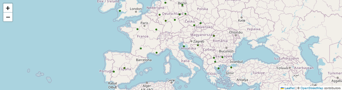
We display the sits.Vec2gdf objects on an interactive map.

• .gdf in green

• .buffer in blue

• .bbox in red

import folium

f = folium.Figure(height=300)
m = folium.Map(location=[45.0, 10], zoom_start=4).add_to(f)
random_pts.gdf.explore(m=m, height=400, color='green')
random_pts.buffer.explore(m=m, height=400)
random_pts.bbox.explore(m=m, height=400, color='red')

2.3. CRS management

In order to request data on a STAC catalog, we need to provide the bounding box coordinates in Lat/Long, i.e the EPSG:4326. Then we also need to specify in which CRS we want to obtain the satellite time series. As we are working in Europe, one of the most appropriate CRS is the EPSG 3035 (ETRS89-extended).

Here we calculate the coordinates in EPSG:4326 and EPSG:3035. Since there are several features (polygons), we keep the coordinates into a dataframe.

# extraction of bbox coordinates in EPSG:4326
bbox_latlong = pd.concat([random_pts.bbox, random_pts.bbox['geometry'].bounds], axis=1)
bbox_latlong['bbox_4326'] = bbox_latlong[['minx', 'miny', 'maxx', 'maxy']].values.tolist()

# extraction of bbox coordinates in EPSG:3035
bbox_3035 = random_pts.bbox.to_crs(3035)
test_3035_bounds = pd.concat([bbox_3035, bbox_3035['geometry'].bounds], axis=1)
test_3035_bounds['bbox_3035'] = test_3035_bounds[['minx', 'miny', 'maxx', 'maxy']].values.tolist()

# concatenation of both coordinates (EPSG:4326 + EPSG:3035)
test_process = pd.concat([bbox_latlong['bbox_4326'], test_3035_bounds['bbox_3035']], axis=1)
test_process['bbox_tuple'] = test_process.apply(lambda row: (row['bbox_4326'], row['bbox_3035']), axis=1)

# quicklook of the output table
test_process.head()

	bbox_4326	bbox_3035	bbox_tuple
0	[8.481383388733258, 49.84437017219194, 8.50138...	[4211764.670013768, 2971302.3517032275, 421324...	([8.481383388733258, 49.84437017219194, 8.5013...
1	[8.402773153496353, 53.135550217099215, 8.4227...	[4214105.200943511, 3337504.924185555, 4215492...	([8.402773153496353, 53.135550217099215, 8.422...
2	[11.166778399392497, 50.00380142653234, 11.186...	[4404616.995128865, 2988598.266294405, 4406085...	([11.166778399392497, 50.00380142653234, 11.18...
3	[23.78724480625752, 40.05894472525313, 23.8072...	[5495790.682699846, 1992060.233281068, 5497840...	([23.78724480625752, 40.05894472525313, 23.807...
4	[16.790197637816156, 48.978094737864616, 16.81...	[4817203.221624014, 2896784.6045746827, 481886...	([16.790197637816156, 48.978094737864616, 16.8...

3. Multiprocessing approach

3.1. How does it work?

If you need to process several points or polygons, we recommand the use of sits.Multiproc() class. This class call in the background the sits.stacAttack() class, distributing the process through the available CPUs.

You can tune the process with the sits.Multiproc().addParams_*() methods:

• Multiproc().addParams_stacAttack(): configure the sits.stacAttack() instance,

• Multiproc().addParams_searchItems(): configure the sits.stacAttack.searchItems() method,

• Multiproc().addParams_loadCube(): configure the sits.stacAttack().loadCube() method,

• Multiproc().addParams_mask(): configure the sits.stacAttack().mask() method.

Then the Multiproc().fetch_func() calls dask.delayed() that is a function that defers execution of Python code, building a task graph for parallel computation. It turns functions/operations into lazy tasks. Multiproc().dask_compute() calls dask.compute() that schedules and runs efficiently (e.g., on multiple cores or a cluster) these operations.

3.2. Producing images from the vector layer

Here is an example of parallelization to produce images that have the same dimensions as the input bounding boxes (see ‘image’ argument). So the output images share only the same spatial resolution. The dimensions (size in x and y) will different.

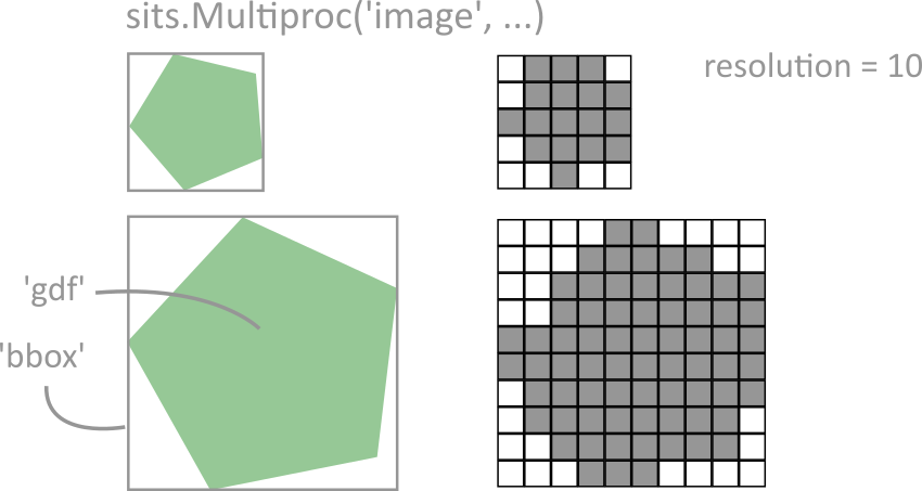
%%time

multi = sits.Multiproc('image', 'nc', data_dir)

multi.addParams_stacAttack(bands=['B03', 'B04', 'B08', 'SCL'])
multi.addParams_searchItems(date_start=datetime(2024, 1, 1),
                            date_end=datetime(2025, 1, 1),
                            query={"eo:cloud_cover": {"lt": 10}})
multi.addParams_loadCube(resolution=20)
multi.addParams_mask(mask_values=[0, 1, 3, 8, 9, 10])

for gid, i in enumerate(test_process['bbox_tuple'][:2]): # here we process only the two first images, remove or modify the slicing
    multi.fetch_func(i[0], i[1], gid, mask=True, gapfill=True)
multi.dask_compute();

3.3. Producing patches from the vector layer

It is also possible to specify the output image size. The option, called “patch”, refers to a small, localized region or segment of an input image. These patches need to be of the same size in deep leaning models to ensure consistent processing, especially in architectures like convolutional neural networks (CNNs) or vision transformers (ViTs).

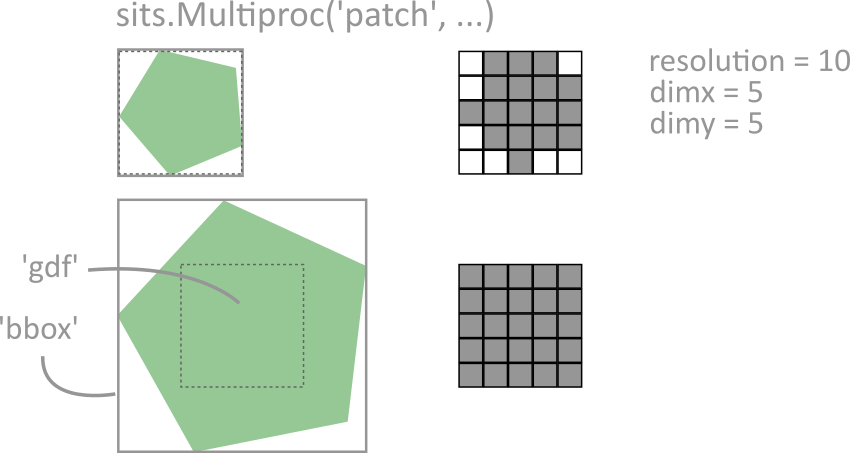
%%time

multi = sits.Multiproc('patch', 'nc', data_dir)

multi.addParams_stacAttack(bands=['B03', 'B04', 'B08', 'SCL'])
multi.addParams_searchItems(date_start=datetime(2024, 1, 1),
                            date_end=datetime(2025, 2, 1),
                            query={"eo:cloud_cover": {"lt": 10}})
multi.addParams_loadCube(dimx=10, dimy=10, resolution=20)
multi.addParams_mask()

for gid, i in enumerate(test_process['bbox_tuple'][:2]): # here we process only the two first patches, remove or modify the slicing
    multi.fetch_func(i[0], i[1], gid, mask=True, gapfill=True)
multi.dask_compute();