Spectral Indices
![]()
Using Banc d’Arguin as an example, we aim to calculate one or more spectral indices. To avoid reinventing the wheel, sits relies on the spyndex package. This package leverages spectral indices from the Awesome Spectral Indices list and provides an expression evaluation method compatible with Python object classes that support overloaded operators (e.g.,
numpy.ndarray, pandas.Series, xarray.DataArray).
1. Installation of SITS package and its depedencies
First, install sits package with pip. We also need some other packages for displaying data.
[1]:
# SITS package
!pip install -q --upgrade sits

# other packages
!pip install -q "dask[dataframe]"
Now we can import sits and some other libraries.
[ ]:
import os
# sits lib
from sits import sits, export
# geospatial libs
import geopandas as gpd
import pandas as pd
import spyndex
# date format
from datetime import datetime
# ignore warnings messages
import warnings
warnings.filterwarnings('ignore')
2. Exploring spectral indices
Scientific literature offers a wide array of spectral indices designed to reveal specific characteristics of objects or phenomena on the Earth’s surface. The Awesome Spectral Indices (ASI) project, initiated in late 2021, catalogs these indices—both well-established and emerging—for optical and radar sensors. Each index is linked to a standardized formula, enabling consistent computation across imagery from various satellites. Furthermore, every index is accompanied by a scientific reference, ensuring transparency and traceability.
The Spyndex package provides seamless access to this library. It offers robust tools to retrieve metadata and efficiently compute spectral indices, streamlining their use in geospatial analyses.
Reference:
Montero, D., Aybar, C., Mahecha, M.D. et al. A standardized catalogue of spectral indices to advance the use of remote sensing in Earth system research. Sci Data 10, 197 (2023). https://doi.org/10.1038/s41597-023-02096-0
2.1. Which indices? Which Spectral bands?
Before loading satellite time series, we need to know which spectral indices we would like to calculate so that we can request the relevant spectral bands. First we list with Spyndex all the available indices.
[3]:
idx_list = spyndex.indices

print(f"number of indices. {len(idx_list)}")
print(F"---\navailable indices:")
print(idx_list)
number of indices. 245
---
available indices:
['AFRI1600', 'AFRI2100', 'ANDWI', 'ARI', 'ARI2', 'ARVI', 'ATSAVI', 'AVI', 'AWEInsh', 'AWEIsh', 'BAI', 'BAIM', 'BAIS2', 'BCC', 'BI', 'BITM', 'BIXS', 'BLFEI', 'BNDVI', 'BRBA', 'BWDRVI', 'BaI', 'CCI', 'CIG', 'CIRE', 'CSI', 'CSIT', 'CVI', 'DBI', 'DBSI', 'DPDD', 'DSI', 'DSWI1', 'DSWI2', 'DSWI3', 'DSWI4', 'DSWI5', 'DVI', 'DVIplus', 'DpRVIHH', 'DpRVIVV', 'EBBI', 'EBI', 'EMBI', 'ENDVI', 'EVI', 'EVI2', 'EVIv', 'ExG', 'ExGR', 'ExR', 'FAI', 'FCVI', 'GARI', 'GBNDVI', 'GCC', 'GDVI', 'GEMI', 'GLI', 'GM1', 'GM2', 'GNDVI', 'GOSAVI', 'GRNDVI', 'GRVI', 'GSAVI', 'GVMI', 'IAVI', 'IBI', 'IKAW', 'IPVI', 'IRECI', 'LSWI', 'MBI', 'MBWI', 'MCARI', 'MCARI1', 'MCARI2', 'MCARI705', 'MCARIOSAVI', 'MCARIOSAVI705', 'MGRVI', 'MIRBI', 'MLSWI26', 'MLSWI27', 'MNDVI', 'MNDWI', 'MNLI', 'MRBVI', 'MSAVI', 'MSI', 'MSR', 'MSR705', 'MTCI', 'MTVI1', 'MTVI2', 'MuWIR', 'NBAI', 'NBLI', 'NBLIOLI', 'NBR', 'NBR2', 'NBRSWIR', 'NBRT1', 'NBRT2', 'NBRT3', 'NBRplus', 'NBSIMS', 'NBUI', 'ND705', 'NDBI', 'NDBaI', 'NDCI', 'NDDI', 'NDGI', 'NDGlaI', 'NDII', 'NDISIb', 'NDISIg', 'NDISImndwi', 'NDISIndwi', 'NDISIr', 'NDMI', 'NDPI', 'NDPolI', 'NDPonI', 'NDREI', 'NDSI', 'NDSII', 'NDSIWV', 'NDSInw', 'NDSWIR', 'NDSaII', 'NDSoI', 'NDTI', 'NDVI', 'NDVI705', 'NDVIMNDWI', 'NDVIT', 'NDWI', 'NDWIns', 'NDYI', 'NGRDI', 'NHFD', 'NIRv', 'NIRvH2', 'NIRvP', 'NLI', 'NMDI', 'NRFIg', 'NRFIr', 'NSDS', 'NSDSI1', 'NSDSI2', 'NSDSI3', 'NSTv1', 'NSTv2', 'NWI', 'NormG', 'NormNIR', 'NormR', 'OCVI', 'OSAVI', 'OSI', 'PI', 'PISI', 'PSRI', 'QpRVI', 'RCC', 'RDVI', 'REDSI', 'RENDVI', 'RFDI', 'RGBVI', 'RGRI', 'RI', 'RI4XS', 'RNDVI', 'RVI', 'S2REP', 'S2WI', 'S3', 'SARVI', 'SAVI', 'SAVI2', 'SAVIT', 'SEVI', 'SI', 'SIPI', 'SLAVI', 'SR', 'SR2', 'SR3', 'SR555', 'SR705', 'SWI', 'SWM', 'SeLI', 'TCARI', 'TCARIOSAVI', 'TCARIOSAVI705', 'TCI', 'TDVI', 'TGI', 'TRRVI', 'TSAVI', 'TTVI', 'TVI', 'TWI', 'TriVI', 'UI', 'VARI', 'VARI700', 'VDDPI', 'VHVVD', 'VHVVP', 'VHVVR', 'VI6T', 'VI700', 'VIBI', 'VIG', 'VVVHD', 'VVVHR', 'VVVHS', 'VgNIRBI', 'VrNIRBI', 'WDRVI', 'WDVI', 'WI1', 'WI2', 'WI2015', 'WRI', 'bNIRv', 'kEVI', 'kIPVI', 'kNDVI', 'kRVI', 'kVARI', 'mND705', 'mSR705', 'sNIRvLSWI', 'sNIRvNDPI', 'sNIRvNDVILSWIP', 'sNIRvNDVILSWIS', 'sNIRvSWIR']
To get details about an index, we can use the following spyndex attributes:
spyndex.indices.[*index short name*]: index’s metadataspyndex.indices.[*index short name*].short_name: Short name of the Spectral Index.spyndex.indices.[*index short name*].long_name: Long name of the Spectral Index.spyndex.indices.[*index short name*].application_domain: Required bands and parameters for the Spectral Index computation.spyndex.indices.[*index short name*].bands: Required bands and parameters for the Spectral Index computation.spyndex.indices.[*index short name*].formula: Formula (as expression) of the Spectral Index.spyndex.indices.[*index short name*].reference: URL to the reference/DOI of the Spectral Index.spyndex.indices.[*index short name*].platforms: Platforms with the required bands for the Spectral Index computation.
For example, we explore here the quite unknown NDVI:
[4]:
print(f"metadata:\n{spyndex.indices.NDVI}")

print(f"---\n short name: {spyndex.indices.NDVI.short_name}")
print(f"---\n long name:{spyndex.indices.NDVI.long_name}")
print(f"---\n application domain: {spyndex.indices.NDVI.application_domain}")
print(f"---\n bands: {spyndex.indices.NDVI.bands}")
print(f"---\n formula: {spyndex.indices.NDVI.formula}")
print(f"---\n reference: {spyndex.indices.NDVI.reference}")
print(f"---\n platform: {spyndex.indices.NDVI.platforms}")
metadata:
NDVI: Normalized Difference Vegetation Index
        * Application Domain: vegetation
        * Bands/Parameters: ['N', 'R']
        * Formula: (N-R)/(N+R)
        * Reference: https://ntrs.nasa.gov/citations/19740022614

---
 short name: NDVI
---
 long name:Normalized Difference Vegetation Index
---
 application domain: vegetation
---
 bands: ['N', 'R']
---
 formula: (N-R)/(N+R)
---
 reference: https://ntrs.nasa.gov/citations/19740022614
---
 platform: ['Sentinel-2', 'Landsat-OLI', 'Landsat-TM', 'Landsat-ETM+', 'MODIS', 'Planet-Fusion']
We will compute three spectral indices:
NDVI,
NDWI, and
BI
All of which include accessible metadata, just like NDVI.
[5]:
print(f"NDWI metadata:\n{spyndex.indices.NDWI}")
print(f"EVI metadata:\n{spyndex.indices.BI}")
NDWI metadata:
NDWI: Normalized Difference Water Index
        * Application Domain: water
        * Bands/Parameters: ['G', 'N']
        * Formula: (G-N)/(G+N)
        * Reference: https://doi.org/10.1080/01431169608948714

EVI metadata:
BI: Bare Soil Index
        * Application Domain: soil
        * Bands/Parameters: ['S1', 'R', 'N', 'B']
        * Formula: ((S1+R)-(N+B))/((S1+R)+(N+B))
        * Reference: http://citeseerx.ist.psu.edu/viewdoc/download?doi=10.1.1.465.8749&rep=rep1&type=pdf
2.2. Selection of spectral bands
We search for all necessary spectral bands to calculate the indices. As the band names are standardized, we need to map them to the Sentinel-2 nomenclature.
[6]:
common_bands = set()
common_bands.update(spyndex.indices.NDVI.bands)
common_bands.update(spyndex.indices.NDWI.bands)
common_bands.update(spyndex.indices.BI.bands)

print("We need to request the following bands:")
print(common_bands)
We need to request the following bands:
{'R', 'N', 'S1', 'G', 'B'}
Spyndex allows us to explore detailed information about spectral bands, including their corresponding names across different naming standards.
[7]:
for band in common_bands:
        print(f"---\nShort name of the Band: {spyndex.bands[band].short_name}")
        print(f" - Description/Name of the Band: {spyndex.bands[band].long_name}")
        print(f" - Common name of the Band according to the EO Ext. Specification for STAC.: {spyndex.bands[band].common_name}")
        print(f" - Minimum wavelength of the spectral range of the band (nm): {spyndex.bands[band].min_wavelength}")
        print(f" - Maximum wavelength of the spectral range of the band (nm): {spyndex.bands[band].max_wavelength}")
        print(f" - Sentinel-2 band name: {spyndex.bands[band].sentinel2a.band}")
---
Short name of the Band: R
 - Description/Name of the Band: Red
 - Common name of the Band according to the EO Ext. Specification for STAC.: red
 - Minimum wavelength of the spectral range of the band (nm): 620
 - Maximum wavelength of the spectral range of the band (nm): 690
 - Sentinel-2 band name: B4
---
Short name of the Band: N
 - Description/Name of the Band: Near-Infrared (NIR)
 - Common name of the Band according to the EO Ext. Specification for STAC.: nir
 - Minimum wavelength of the spectral range of the band (nm): 760
 - Maximum wavelength of the spectral range of the band (nm): 900
 - Sentinel-2 band name: B8
---
Short name of the Band: S1
 - Description/Name of the Band: Short-wave Infrared (SWIR) 1
 - Common name of the Band according to the EO Ext. Specification for STAC.: swir16
 - Minimum wavelength of the spectral range of the band (nm): 1550
 - Maximum wavelength of the spectral range of the band (nm): 1750
 - Sentinel-2 band name: B11
---
Short name of the Band: G
 - Description/Name of the Band: Green
 - Common name of the Band according to the EO Ext. Specification for STAC.: green
 - Minimum wavelength of the spectral range of the band (nm): 510
 - Maximum wavelength of the spectral range of the band (nm): 600
 - Sentinel-2 band name: B3
---
Short name of the Band: B
 - Description/Name of the Band: Blue
 - Common name of the Band according to the EO Ext. Specification for STAC.: blue
 - Minimum wavelength of the spectral range of the band (nm): 450
 - Maximum wavelength of the spectral range of the band (nm): 530
 - Sentinel-2 band name: B2
Unfortunately, the Sentinel-2 band names don’t align perfectly with those used in the STAC catalog of the Microsoft Planetary Computer, so we need to map them manually.
[8]:
band_mapping = {'B': 'B02', 'G': 'B03', 'R': 'B04', 'N': 'B08', 'S1': 'B11'}
3. Loading the sentinel-2 time series
3.1. Data loading
The geojson vector file describing the position of the sandbank is stored in the Github repository. We download it into our current workspace.
[9]:
!mkdir -p test_data
![ ! -f test_data/banc_arguin.geojson ] && wget https://raw.githubusercontent.com/kenoz/SITS_utils/refs/heads/main/sits/data/banc_arguin.geojson -P test_data
We load the vector file, named banc_arguin.geojson, as a geoDataFrame object with the sits method: sits.Vec2gdf().
[10]:
data_dir = 'test_data'

# Load vector
v_arguin = sits.Vec2gdf(os.path.join(data_dir, 'banc_arguin.geojson'))

# Define polygon bounding box
v_arguin.set_bbox('gdf')

# CRS management
bbox_4326 = list(v_arguin.bbox.iloc[0]['geometry'].bounds)
bbox_3035 = list(v_arguin.bbox.to_crs(3035).iloc[0]['geometry'].bounds)
3.2. Loading and preprocessing of a Satellite Image Time-Series (SITS)
In this example, we have only one area (one polygon) to process. We use the class sits.StacAttack to request and preprocess the data. The request consists in retrieving Sentinel-2 images (level 2A) acquired from January 1, 2016 to January 1, 2025 with cloud cover less than 10%. Then we build a 4 bands geo-datacube (‘B03’, ‘B04’, ‘B08’ and ‘SCL’) in EPSG:3035 with a 20m spatial resolution.
[11]:
# instance of the class sits.StacAttack()
ts_S2 = sits.StacAttack(provider='mpc',
                        collection='sentinel-2-l2a',
                        bands=['B02', 'B03', 'B04', 'B08', 'B11', 'SCL'])

# search of items based on bbox coordinates and time interval criteria
ts_S2.searchItems(bbox_4326,
                  date_start=datetime(2016, 1, 1),
                  date_end=datetime(2025, 1, 1),
                  query={"eo:cloud_cover": {"lt": 10}}
                 )
# load of the time series in a lazy way
ts_S2.loadCube(bbox_3035, resolution=20, crs_out=3035)

ts_S2.cube
[11]:
<xarray.Dataset> Size: 277MB
Dimensions:      (y: 517, x: 413, time: 108)
Coordinates:
  * y            (y) float64 4kB 2.459e+06 2.459e+06 ... 2.448e+06 2.448e+06
  * x            (x) float64 3kB 3.426e+06 3.426e+06 ... 3.435e+06 3.435e+06
  * time         (time) datetime64[ns] 864B 2016-03-18T11:11:02.030000 ... 20...
    spatial_ref  int64 8B 0
Data variables:
    B02          (time, y, x) uint16 46MB dask.array<chunksize=(1, 517, 413), meta=np.ndarray>
    B03          (time, y, x) uint16 46MB dask.array<chunksize=(1, 517, 413), meta=np.ndarray>
    B04          (time, y, x) uint16 46MB dask.array<chunksize=(1, 517, 413), meta=np.ndarray>
    B08          (time, y, x) uint16 46MB dask.array<chunksize=(1, 517, 413), meta=np.ndarray>
    B11          (time, y, x) uint16 46MB dask.array<chunksize=(1, 517, 413), meta=np.ndarray>
SCL (time, y, x) uint16 46MB dask.array<chunksize=(1, 517, 413), meta=np.ndarray>4. Computing spectral indices
Spyndex’s index computation capabilities are directly embedded in the sits package via the sits.StacAttack class. Below, we demonstrate how to apply sits to compute one or more spectral indices from satellite time series data.
4.1. Computing the NDVI
The method sits.StacAttack.spectral_index allows us to compute one or more indices.
[12]:
ts_S2.spectral_index('NDVI', band_mapping)
Here, we produce a xarray.Dataset with NDVI as a variable.
[13]:
ts_S2.indices
[13]:
<xarray.Dataset> Size: 184MB
Dimensions:      (y: 517, x: 413, time: 108)
Coordinates:
  * y            (y) float64 4kB 2.459e+06 2.459e+06 ... 2.448e+06 2.448e+06
  * x            (x) float64 3kB 3.426e+06 3.426e+06 ... 3.435e+06 3.435e+06
  * time         (time) datetime64[ns] 864B 2016-03-18T11:11:02.030000 ... 20...
    spatial_ref  int64 8B 0
Data variables: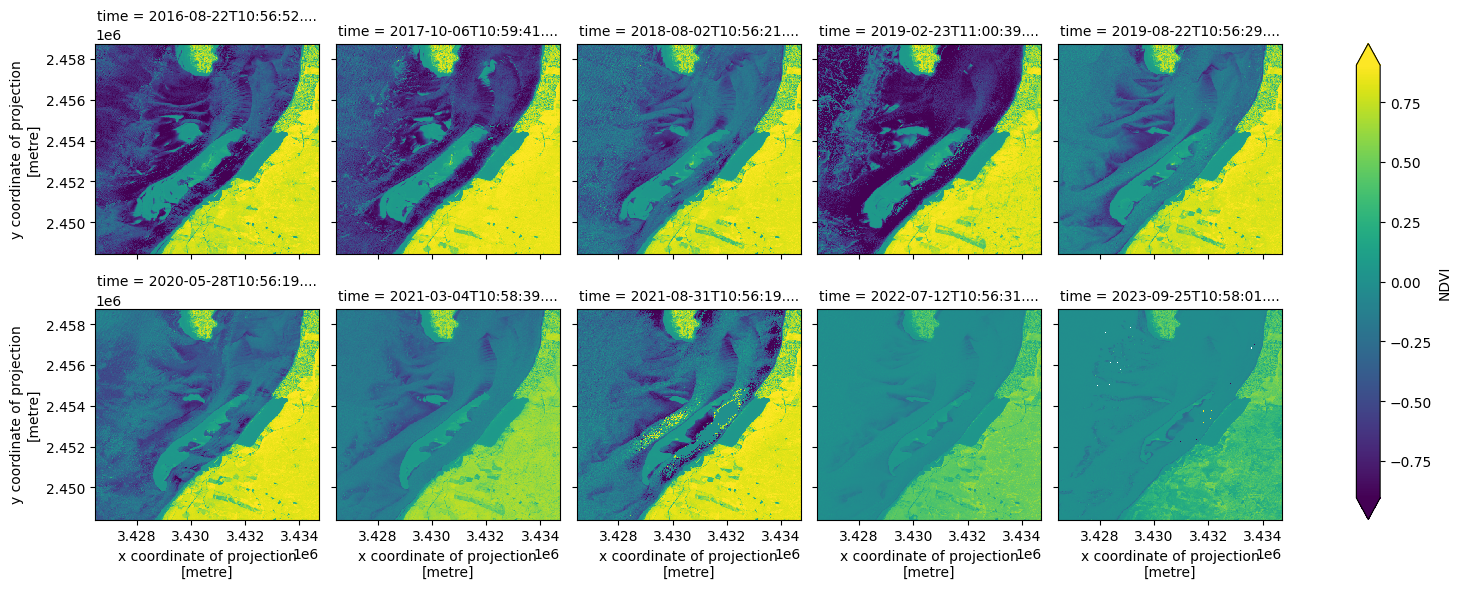
NDVI (time, y, x) float64 184MB dask.array<chunksize=(1, 517, 413), meta=np.ndarray>The NDVI time series is plotted here with a sampling interval of 10 images. The index was derived directly from spectral bands, without masking or interpolating missing values.
[14]:
ts_S2.indices.NDVI[8::10].plot.imshow(col_wrap=5, col="time", cmap='viridis', robust=True, size=3)
[14]:
<xarray.plot.facetgrid.FacetGrid at 0x7f403f11bf10>
4.2. Computing a list of indices
The sits.StacAttack.spectral_index method accepts a list of indices, allowing simultaneous computation of several spectral indices instead of just one.
[15]:
ts_S2.spectral_index(['NDVI', 'NDWI', 'BI'], band_mapping)
Here, we produce a xarray.Dataset that stores indices as variables.
[16]:
ts_S2.indices
[16]:
<xarray.Dataset> Size: 553MB
Dimensions:      (y: 517, x: 413, time: 108)
Coordinates:
  * y            (y) float64 4kB 2.459e+06 2.459e+06 ... 2.448e+06 2.448e+06
  * x            (x) float64 3kB 3.426e+06 3.426e+06 ... 3.435e+06 3.435e+06
  * time         (time) datetime64[ns] 864B 2016-03-18T11:11:02.030000 ... 20...
Data variables:
    NDVI         (time, y, x) float64 184MB dask.array<chunksize=(1, 517, 413), meta=np.ndarray>
    NDWI         (time, y, x) float64 184MB dask.array<chunksize=(1, 517, 413), meta=np.ndarray>
    BI           (time, y, x) float64 184MB dask.array<chunksize=(1, 517, 413), meta=np.ndarray>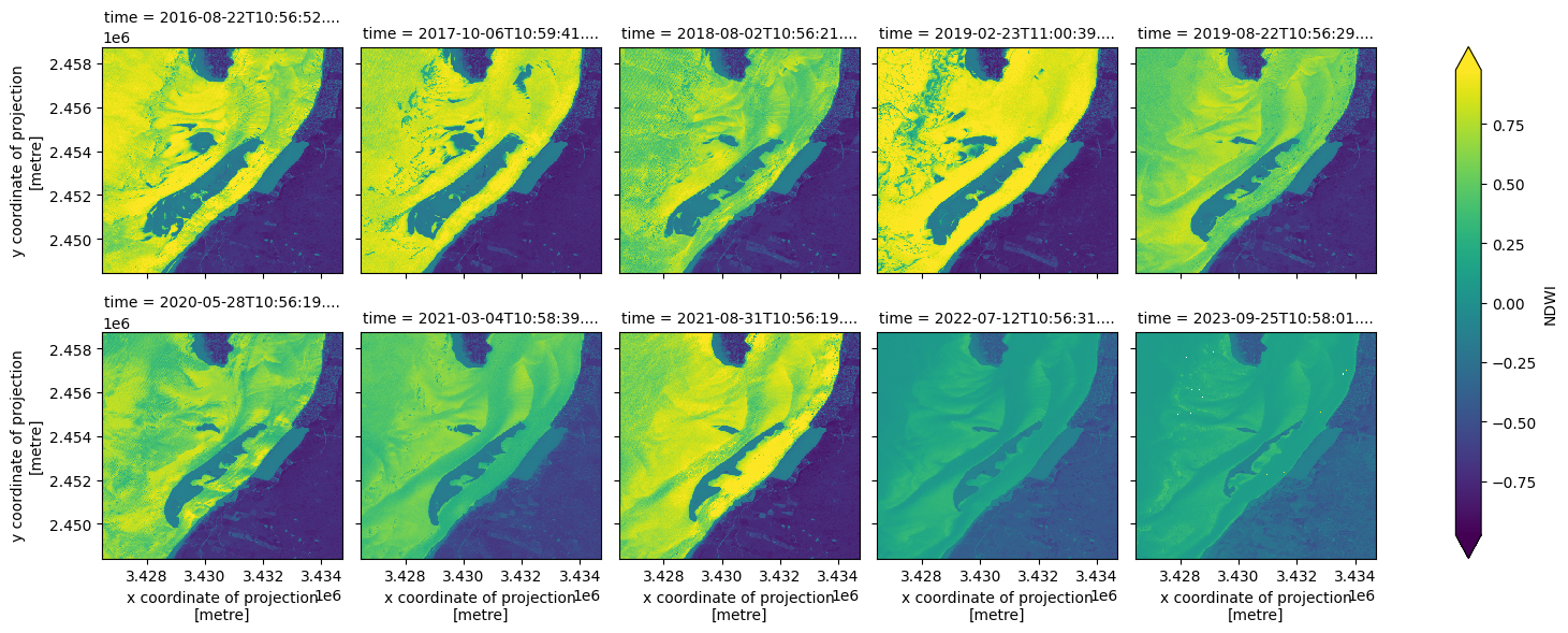
spatial_ref int64 8B 0The NDWI time series is plotted here with a sampling interval of 10 images. The index was derived directly from spectral bands, without masking or interpolating missing values.
[17]:
ts_S2.indices.NDWI[8::10].plot.imshow(col_wrap=5, col="time", cmap='viridis', robust=True, size=3)
[17]:
<xarray.plot.facetgrid.FacetGrid at 0x7f4037c35210>
4.3. Saving Indices as a NetCDF file
To save images, just write the following instruction:
[18]:
ts_S2.to_nc(data_dir, cube='indices')
5. Spectral indices with multiprocessing
5.1. Data loading
The GeoJSON vector file, available in the GitHub repository, contains 24 sampling points distributed across Europe. For a detailed explanation of the pre-processing steps, refer to the dedicated section in the second notebook.
[19]:
!mkdir -p test_data
![ ! -f test_data/rand_pts.geojson ] && wget https://raw.githubusercontent.com/kenoz/SITS_utils/refs/heads/main/data/rand_pts.geojson -P test_data

random_pts = sits.Vec2gdf(os.path.join(data_dir, 'rand_pts.geojson'))
random_pts.gdf.head()

# buffer distance of 0.01 degree (1.11 km approx.)
random_pts.set_buffer('gdf', 0.01)

# bbox of buffer polygon
random_pts.set_bbox('buffer')

# extraction of bbox coordinates in EPSG:4326
bbox_latlong = pd.concat([random_pts.bbox, random_pts.bbox['geometry'].bounds], axis=1)
bbox_latlong['bbox_4326'] = bbox_latlong[['minx', 'miny', 'maxx', 'maxy']].values.tolist()

# extraction of bbox coordinates in EPSG:3035
bbox_3035 = random_pts.bbox.to_crs(3035)
test_3035_bounds = pd.concat([bbox_3035, bbox_3035['geometry'].bounds], axis=1)
test_3035_bounds['bbox_3035'] = test_3035_bounds[['minx', 'miny', 'maxx', 'maxy']].values.tolist()

# concatenation of both coordinates (EPSG:4326 + EPSG:3035)
test_process = pd.concat([bbox_latlong['bbox_4326'], test_3035_bounds['bbox_3035']], axis=1)
test_process['bbox_tuple'] = test_process.apply(lambda row: (row['bbox_4326'], row['bbox_3035']), axis=1)
5.2. Producing indices patches from the vector layer
To compute one or more spectral indices over patches, follow these steps:
Use
Multiproc().addParams_spectral_index()to configure thesits.stacAttack().spectral_index()method.Set the
indicesparameter toTruewhen callingMultiproc().fetch_func(i[0], i[1], gid, indices=True).
[ ]:
multi = sits.Multiproc('patch', 'nc', data_dir)

multi.addParams_stacAttack(bands=['B02', 'B03', 'B04', 'B08', 'B11', 'SCL'])
multi.addParams_searchItems(date_start=datetime(2024, 1, 1),
                            date_end=datetime(2025, 2, 1),
                            query={"eo:cloud_cover": {"lt": 10}})
multi.addParams_loadCube(dimx=10, dimy=10, resolution=20)
multi.addParams_spectral_index(['NDVI', 'NDWI', 'BI'], band_mapping)

for gid, i in enumerate(test_process['bbox_tuple'][:2]): # here we process only the two first patches, remove or modify the slicing
    multi.fetch_func(i[0], i[1], gid, indices=True)
multi.dask_compute();